1. Introduction to Mathematics for Machine Learning

Aspiring Machine Learning Engineers often tend to ask “What is the use of Mathematics for Machine Learning when we have computers to do it all?”. Well, that is true. Our computers have become capable enough to do the math in split seconds where we would take minutes or hours to perform the calculations. But in reality, it’s not the ability to solve the math. Rather, it is the eye of how the math needs to be applied.

You need to analyze the data and infer information so that you can create a model that learns from the data. Math can help you in so many ways that it becomes mind-boggling that someone could hate this subject. Of course, doing math by hand is something I hate too but knowing how I use math is enough to explain my love for math.

Allow me to extend this love to you guys too because I won’t be teaching you just the Mathematics for Machine Learning but the various applications you can use it for, in real life!

2. Linear Algebra

The chart below will help you understand rather easily that Linear Algebra is used most widely when it comes to Machine Learning. It covers so many aspects making it unavoidable if you want to learn Mathematics for Machine Learning.

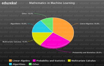
Linear Algebra helps you in optimizing data, operations that can be performed on pixels such as shearing, rotation and much more. You can understand why Linear Algebra is such an important aspect when it comes to Mathematics for Machine Learning.

Let’s start off with the Mathematics for Machine Learning now and understand as much as we can. Remember that no one can master anything in a go. It takes time, patience and real-world experiences to help you master math but this article will for sure help you out with the basics!

2.1 Scalar

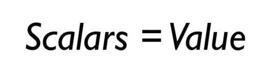
What do we understand by a scalar? To put it in simple words, Scalars are just values that represent something. It can be something like the size of a house to temperature in an engine, scalars help us represent them and their values. So the math in scalars? Just simple Arithmetic.

Let me give you a small example so that you understand what I’m trying to mean by that. Let me take the example of a laptop on sale:

• Suppose a Laptop costs around 50,000 Rupees and it is on a Sale for 50%. That means it is half the price and you calculate the price by dividing by 2:

50,000 / 2 = 25,000

• If you want to buy 5 of the same laptops which are on sale, you just multiply by 5:

25,000 X 5 = 1,25,000

• You want to buy accessories with the laptop, you add their particular values:

25,000 + 1000 = 26,000

• And if you don’t want the accessory, just remove their value from the total:

26,000 – 1000 = 25,000

That is in simple words, a Scalar. Simple arithmetic and nothing fancy. That is all you would need to know about Scalars. Let’s move over to Vectors in our article of Mathematics for Machine Learning!

2.2 Vectors

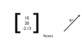
Vectors can get a bit complicated, as they are different for different backgrounds.

• Computer Science people can interpret Vectors as a list of numbers that represent something.

• Physicists consider Vectors to be a scalar with a direction and it is independent of the plane.

• Mathematicians take Vectors to be a combination of both and try to generalize it for everyone.

All of these standpoints are absolutely correct and that’s what makes it so confusing for anyone learning about Linear Algebra for Mathematics for Machine Learning.

In Machine Learning, we usually consider Vectors in the standpoint of a Computer Scientist when the data is tabular consisting of rows and columns. When our data is in the form of pixels (pictures), we consider them as Vectors that are bound to the origin and transform them to Matrices and perform operations that we shall discuss later.

Now that we have a brief idea about Vectors, let’s jump over to the operations that you need to know when working with Vectors.

2.3 Vector Operations

Operations on Vectors can be applied only when you know what kind of data you are working with. Suppose you have pixel data and want to apply rotations but end up doing something wholly different, your model will not work because it is doing the wrong operations here. So make sure that you know what you are working with, only then apply the required operations.

• Vector Addition (Dot Product)

This operation is the addition of two vectors, but it is not just simple arithmetic. It is actually the displacement that we achieve from the working of both these vectors. The below diagram will help you understand this better.

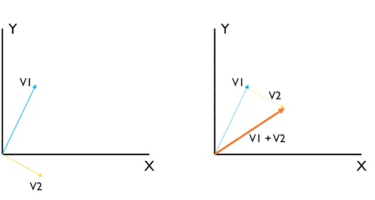
You can see that we had 2 vectors V1 and V2 and to add them, add their effect together. For example, if V1 has values [1, 2] and V2 has values [1, -1] for the X and Y axis respectively, the effective V1+V2 will have the value [2, 1] which is to add the scalar values of the Vectors. This is also called as the Dot Product.

The Equation for Dot Product is ^A.^B = a1+b1, a2+b2, …

• Scalar Multiplication

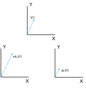
If a Vector is multiplied with a constant, it either grows or shrinks accordingly. This can be used in something called as Shearing which helps in the manipulation of pixel information.

The Equation for Scalar Multiplication is +k.^A or -k.^A = ^A’

The below diagrams will help you understand how this works.

With that, let’s move over to Projections in our article of Mathematics for Machine Learning.

Projection of a Vector onto Another

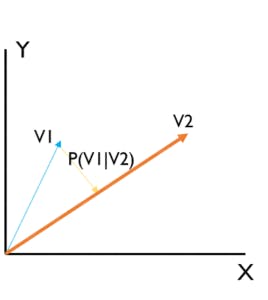
The projection of a vector onto another is what we are calculating here. Projections help to find the shadows of a pixel. They can be then used to find the length, distance and map a 2D object to a 3D object for better analysis.

The Equation goes like this: Proj(^V1 on ^V2) = ^V1.(^V2 / |^V2|)

2.4 Matrix

What is a matrix? Think of 2 equations. Let’s say,

2x + 2y = 10 — eqn.1

4x + y =18 — eqn.2

If we Multiply eqn.1 with 2 and eqn.2 with -1, then by simplification, we get the results as,

4x + 4y = 20

-4x – y = -18

Leading us to,

3y = 2 -> y = ⅔

x = 13/3

The equation does not have to be this difficult, but, think if there was a simpler way to do all of this. This is where Matrices come into the picture.

So the above Equations can be represented as:

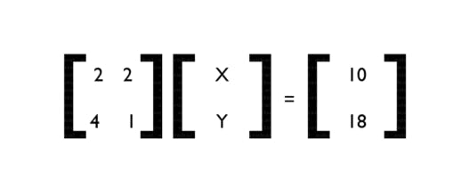
Then it becomes very easy to solve the problem. We can use Matrix Operations to solve the problem efficiently. But why are matrices so important? That’s because they are something which we can use to represent in our computers.

Functions represent Data in a generalized form. That is the reason they are so essential to understand. These functions can then be solved to obtain coordinates where we can then use them for something else depending on the application.

Just for your knowledge, make sure you go through the types of Matrices. I have listed a few below:

• Row Matrix: Has one 1 row and many columns
• Column Matrix: Has 1 column and many rows
• Square Matrix: Number of rows and columns are equal
• Diagonal Matrix: Only diagonal elements are values, others are zero
• Identity Matrix: The matrix has all elements as 1’s
• Sparse Matrix: Very few values in the Matrix

• Dense Matrix: Many values in the Matrix

  Now that we understand what Matrix is and some of the important types, let’s look at the Operations in Matrices in our article of Mathematics for Machine Learning.

2.5 Matrix Operations

There are various operations that can be done on a Matrix:

• Matrix Addition
• Matrix Multiplication
• Transpose
• Determinant
• Inverse

Let’s understand all of them now!

• Matrix Addition

Matrix Addition is the simple process of adding the corresponding elements of 2 Matrices. It is as simple as that. C = A + B where A and B are 2 Matrices.

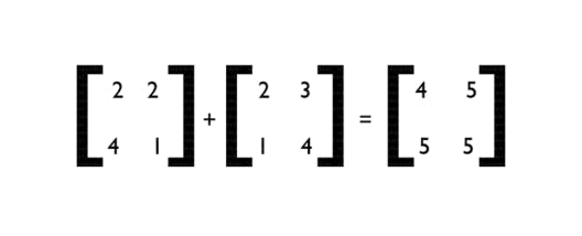
That’s how simple Matrix Addition is! Let’s move over to Matrix Multiplication.

• Matrix Multiplication

Matrix Multiplication is to multiply the rows and columns of 2 Matrices accordingly. To be specific, multiply the elements of the 1st row of Matrix 1 with the columns of Matrix 2.

The equation goes like C = A x B

Considering that A and B are both of order 2, which means they both have 2 rows and 2 columns, then the in-depth equation is as follows:

C = [[a11b11+a12b21 a11b12+a12b22] [a21b11+a22b21 a21b12+a22b22]]

That is how the Matrix Multiplication takes place. Let me show you an example to help you understand better.

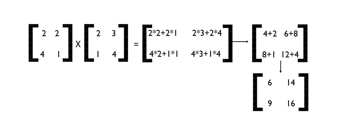
You need to know that Matrix Multiplication can be carried out only if the count of rows of Matrix 1 is equal to the count of columns of Matrix 2. If they are not, you will not be able to perform the matrix multiplication. With that, let’s understand the transpose of a Matrix in our article of Mathematics for Machine Learning.

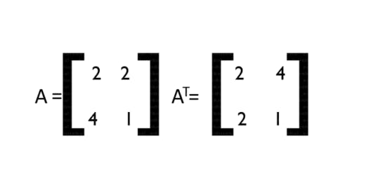
• Transpose of a Matrix

The transpose of a Matrix is the interchanged rows and columns that result in a new Matrix. Transpose can be used to flip the dimensions of a Matrix or Pixel which represent information.

The transpose of a Matrix is denoted by a subscript T. Shown below is an example of Matrix Transpose.

So now that we have understood the Transpose, let’s understand the Determinant of a Matrix.

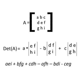
• Determinant of a Matrix

The Determinant of a Matrix is the value of a Matrix, specifically, it tells you the Scalar of a Matrix. The determinant gives you the product of the Eigenvalues in the Matrix. The Determinant can be found by the following operation:

• Inverse of a Matrix

The inverse of a matrix is such that when a Matrix is multiplied with it, it gives us back an Identity Matrix. But, when is this useful? It is when we are solving equations and applying transformations to our matrices. How do we find the Inverse of a Matrix? It’s really simple.

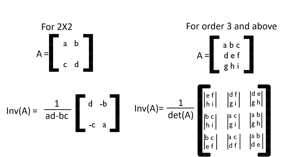
In some cases, Matrices do not have an Inverse. Which means that it is not possible to determine the value as the matrix does not have sufficient data to help us find the inverse.

So this brings us to the end of the operations that we would need for Machine Learning. Next, let’s move over to see how these vectors and matrices map with each other.

2.6 Vectors as Matrices

Vectors can have either 2 or 3 components along with some angle from the origin. This can be easily translated into Matrices. It can then be used to perform three of the most well-known applications that we have, when it comes to pixel data.

We can perform Scaling, Rotation and Shearing on the pixel data. Make an algorithm that can learn factors of the pixels and perform better when it comes to getting output.

For example, let’s say vector V1 = 3x + 4y and vector V2 = x + 2y. How do we transform them into matrices? If you would have given a close look at the operations, I have already used this concept to obtain an answer in Matrix Introduction.

So, these vectors are simply translated into:

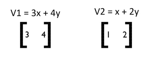
It is really simple to apply transformations on them now because they are now in the form of Matrices. The following matrices are used to apply the transformation on them.

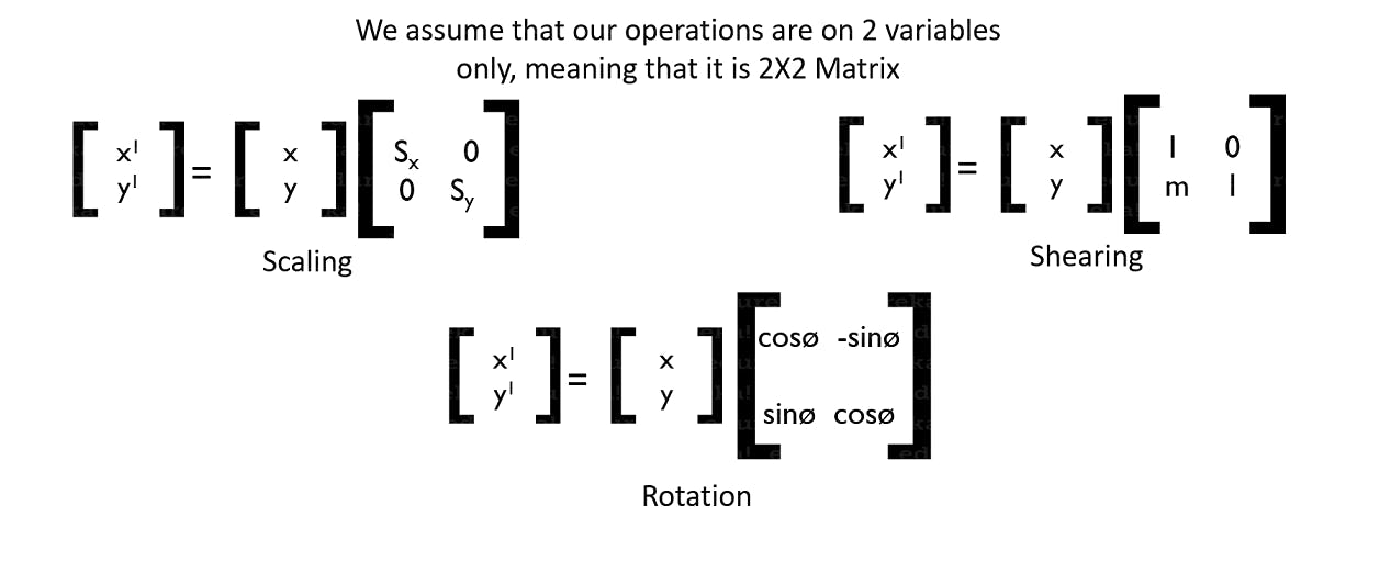
The scaling matrix scales the vector and makes it small or big. The shearing will change the vector by a particular side or co-ordinate. The rotation is rotating the vector around the origin according to the values provided.

These are really simple to implement when we have our vector in the matrix form. Hence the convergence of these two kinds. So now that we are okay with Vectors and Matrices, let’s look at the two most important ways to solve equations which are:

1. Row Echelon Method
2. Inverse Method

Let’s understand them in depth.

• 1. Row Echelon Method Let’s take some vectors in their linear equation form which go like,

2x + y – z = 2

x + 3y + 2z = 1

x + y + z = 2

So now, let’s take them into the matrix form where we obtain:

[[2 1 -1 2]

[1 3 2 1]

[1 1 1 1]]

Let’s reduce it into the Echelon Form:

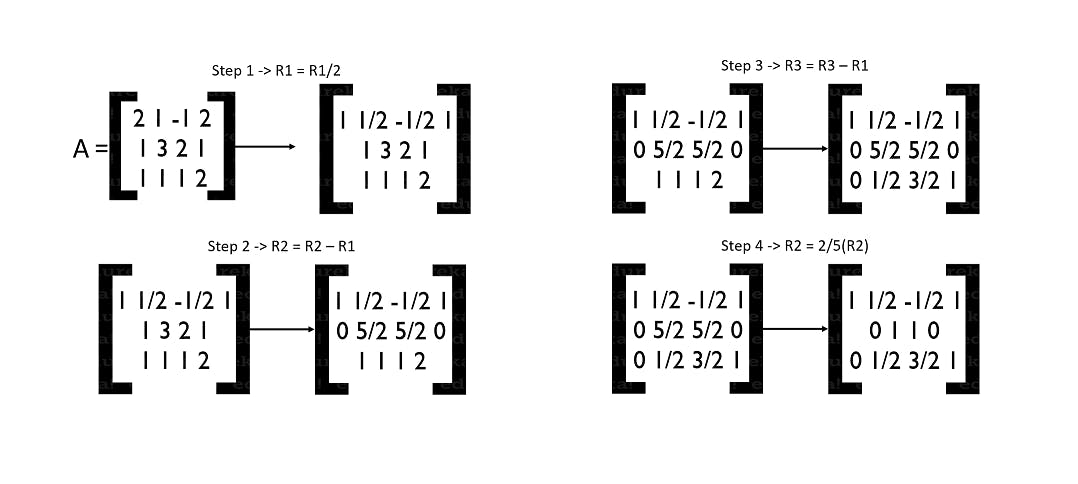
We have now finished reducing our matrix into its echelon form. But what was the use of it? Well, you may have not noticed it or you may have but we have already solved the equation. Yes, our equation has been solved and we have the values of x, y, z.

If we take a closer look and convert the matrix back into the equation, we shall obtain:

x = 2

y = -1

z = 1

So that is a simple example of how we can solve and find the values of the vectors. Isn’t that cool? There is another way to do the same by finding the Inverse. Let’s go for that now in our article of Mathematics for Machine Learning!

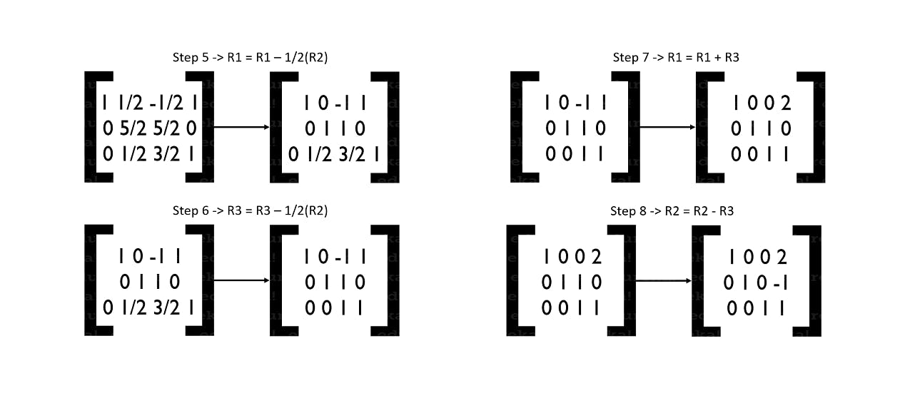
• 2. Inverse Method So let’s take some vectors in their equation form. For example,

4x + 3y = -13

-10x – 2y = 5

This in its matrix form will be:

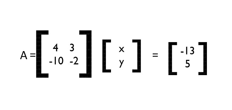
Now, let me show you the equations of how this actually works.

We know by now that,

A.B = C

Thus if we multiply both sides with the Inverse of A, it shouldn’t change the values of the equation right? We get,

A-1.[A.B] = A-1.C

Now if we assume that B is the matrix whose values we are to find, it becomes easy for us as A and A-1 cancel out each other and give us an Identity Matrix. We are then left with,

B = A-1.C

So, let’s use this logic and find the values of x and y.

We have already set our equation in that form. Let’s solve!

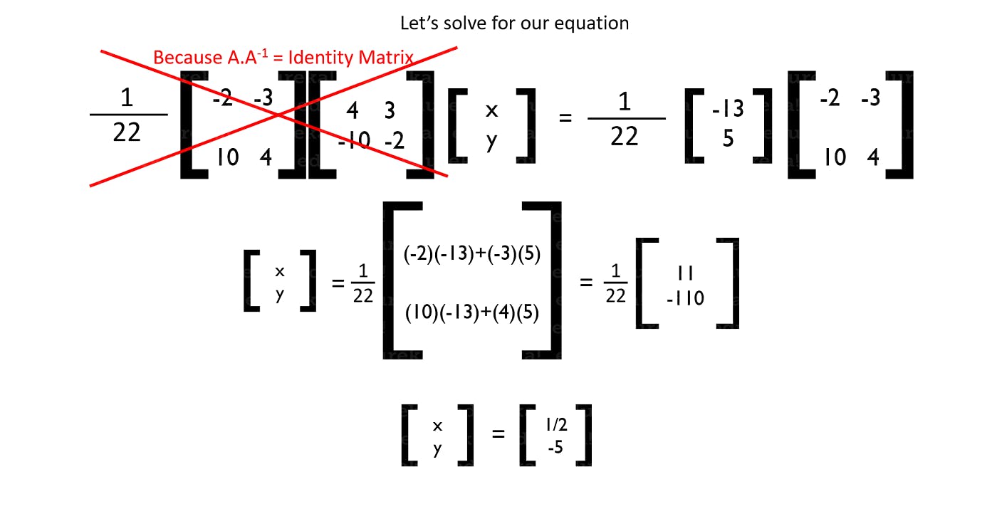
So from this method, we were able to find the values of our x and y very easily. These methods come in really handy when we need to solve for the coordinates of our vectors and much more. That is all you would need to know to get started with Machine Learning. You could definitely go in-depth with these concepts but for our requirement, this is sufficient.

By now, I expect you guys to understand what exactly are Vectors and Matrices along with their operations so that we can further our study. We now move over to EigenVectors and EigenValues.

Eigen Vectors

What are EigenVectors and EigenValues? Let me explain that to you guys with a simple example.

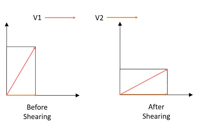
Suppose we have a rectangle in which we have 2 vectors V1 and V2 which help us describe this rectangle. Simple enough to understand, right? Now, what if we apply the shearing operation on this rectangle?

You can see that the vectors V1 and V2 scale in their size but there’s something much more than meets the eye. The vector V1 has also moved its direction. But that is not the case with our vector V2. Even though the scaling of V2 has changed, the direction has not.

No matter you apply scaling or shearing operations, the direction of this vector V2 shall not change and that is what makes V2 an EigenVector. So what’s an EigenValue? It’s the list of factors by which the vector transformations do not affect the direction of the EigenVector.

Putting it to a definition, EigenVectors are those vectors that do not change its direction even if transformation is applied to them. The list of values by which the transformations are applied on the EigenVector and make sure that the direction does not change is the EigenValues.

I hope this helps you understand what an EigenVector and EigenValue is. But what is the significance of the EigenVector? What real purpose do they serve us? Let’s discuss them in the next section of the article.

2.7 Application of Linear Algebra in Machine Learning

Now that we have discussed so much about Linear Algebra, the main question is how do we use all of this? Let’s find the answer to this question now.

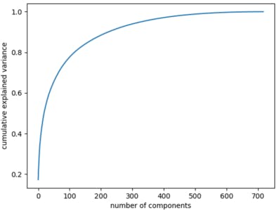
• Principal Component Analysis (PCA) is one of the most important techniques that utilize Linear Algebra in-depth. The main motive behind PCA is to reduce the dimensionality of the data using Eigen Decomposition and Matrices. As you can see in the graph below, the variance increases as the components increase, so PCA eliminates the variance.

• When you work with images, you can use the concepts of Linear Algebra to scale, smoothen, crop and much more. You have predefined operations or you can create such operations that can take care of all this. You can make use of NumPy arrays and load image data, later make use of the operations to do your work.

• Encoding Datasets is another application where Linear Algebra is used. You have in-built functions in many languages that help you encode strings to characters or something else. These functions are made using Linear Algebra.

• You may know about optimizing the outputs so that we can get the most optimum values needed by our model. There is mostly the use of Multivariate Calculus but there are certain times when even Linear Algebra equations and more can be used to optimize our model and their weights that yield outputs.

• Singular Value Decomposition (SVD) is another application which is of the same kind of PCA but for single dimensions. This helps in the reduction of noise, helps improve the quality of the information that is obtained from the dimension and so on. It uses EigenVectors and Matrix Factorizations (Matrix Operations) for the working.

• Images can be altered and new images can be made from them. We use the advanced concepts of Shadow, Projection etc. in a Neural Network that transforms the pixels to obtain alternate images of that image. It is capable of transforming 2D objects to 3D which requires Linear Algebra.

• Latent Semantic Analysis uses Sparse Matrices Factorization with the SVD to give you the most important parts of the text document. These can be used for Natural Language Processing. Deep Learning needs Linear Algebra because it works on optimizations and more to give the best possible output.

3. Multivariate Calculus

Multivariate Calculus is one of the most important parts of Mathematics for Machine Learning. It helps us in solving the second most important problem that we face in developing Machine Learning models. The first problem obviously being the pre-processing of data, the next being the optimization of the model.

This helps us to optimize and increase the performance of our model and gives us some of the most reliable results. So how does something, that almost half of the class hated, help us to solve such a problem? Let’s break all the ice surrounding this. But before that, we need to understand the basics. So let’s calculus! :D

3.1 What is Differentiation?

Differentiation is breaking down the function into several parts so that you can understand every element and analyze it in-depth. They are helpful in finding the sensitivity of a function to the varying inputs. A good function gives a good output which can be described using a rather easy equation. The same cannot be said for a bad function.

Below are a set of graphs that describe what exactly are good-bad functions and their corresponding equations.

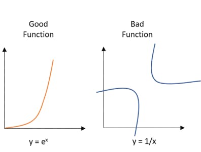
If you take a close look here, it is really easy to break the function of y=ex, whereas it is much more difficult to break y=1/x because the function behaves differently for different inputs. So, we can say that ex is much more efficient when it comes to varying inputs but the same cannot be said for 1/x.

Now, what was the use of all that? Yeah, we know which data is sensitive and which is not. To know what we are doing, we need to learn all the basics of differentiation to understand what we are trying to do.

So, let’s start with the basics now. Let us derive the differentiation formula for now.

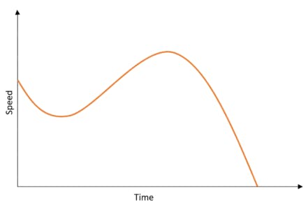
Let’s assume that we have a car moving in a single direction only and is already in motion. If we plot a graph of its Speed vs. Time, it communicates to us how the speed varies as the time keeps increasing and halts after a certain point. Now if we want to know the rate at which the speed varies with respect to time, it turns out that we are actually finding the acceleration. The acceleration of the car can then be plotted as follows:

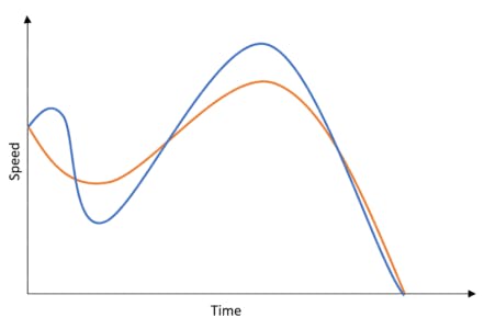
What this means is that Acceleration is actually a derivative of Speed because the speed we have here is just magnitude and does not hold more factors for simplification. If there was no Speed, there would be no acceleration too.

Now that we have acceleration, we can justify whether the car had a varying or constant change in the speed it was moving it and much more that we would want to find. But in this case, that is all we will need.

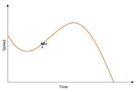
Now, think that you want to find the change in acceleration between a certain range in the time span. We mark 2 points ‘x’ and some variable which is a small portion more than ‘x’. We can denote this as ‘x+Δx’. Let’s denote this on the graph here:

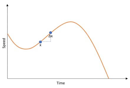
Now we know that this range has many values in between them. But what if we want to know the rate of change only between one point and the next. We know that is really kind of impossible because, between a range, there are countless numbers as the function is continuous. Thus we approximate that the limit or the step between two input variables is 0.

Remember that this 0 that we are assuming is only the smallest possible value that we can make up and not the absolute 0. If we ever work with the absolute 0, we would never have had any function, to begin with.

If you are still confused, this zero is basically some value of 0.00000…… and some numbers ahead, but never really zero. That is the only way we can put this as. So now that we have understood what we are really trying to find, let’s make it a general equation. Let’s derive the Derivation Formula.

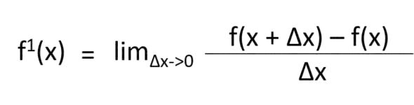
That is how the formula comes into existence. This helps us find the rate of change between one point to the other. It is such an important concept as it plays a huge role in the optimization of Machine Learning models.

You need to understand that this is the first order of differentiation only. If we differentiate the output of the first differentiation, it becomes the second-order differentiation and so on. That is all the introduction we needed from Differentiation.

3.2 Rules of Differentiation

Now that we have derived the basic formula of Derivation, let’s understand some of the most important rules that we have in Differentiation. I will also show how the rule comes into existence. The rules we discuss here are:

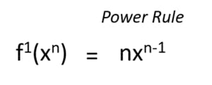
• Power Rule
• Sum Rule
• Product Rule
• Chain Rule

• Power Rule

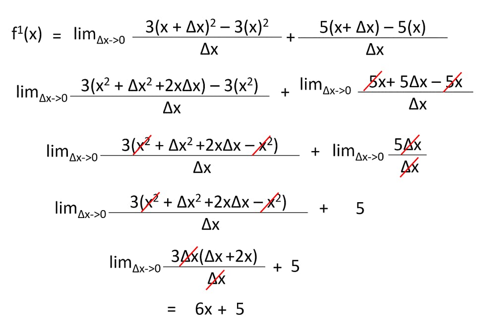
Let’s understand the power rule using the derivation formula that we have. Suppose we have a function f(x) = 3x2. We need to find the derivative of this. So what do we do? Let’s put this into the equation and solve it.

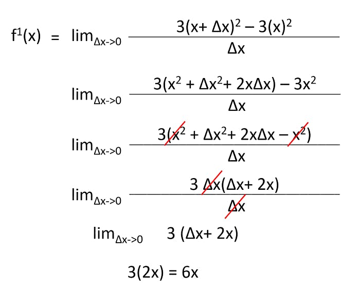
That is how we solve the problem using our derivation function. On observation of solutions on such, we found a common pattern and hence we deduced the chain rule which goes as follows. These rules help in solving the problem faster and more efficiently.

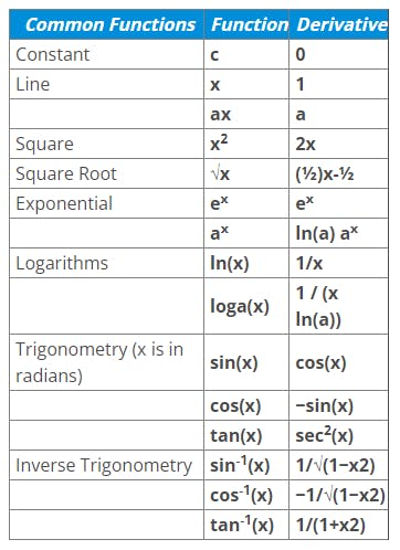
Whenever you encounter such problems, just use the power rule and solve it in a jiffy. For some problems, you won’t be able to use this rule and so it has its own way of solving. I will list down the most common functions in a table for your reference at the end of this section.

• Sum Rule

The sum rule is very straight-forward in what it is trying to communicate. If the variables are split down with addition signs between them, then the derivative is just the addition of the derivatives of the variables. Let’s solve a problem and derive the sum rule.

Suppose we have an equation, f(x) = 3x2 + 5x.

This means that the sum rule can now be defined as the following:

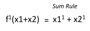
That is what the sum rule is all about. It is as simple as that. We can also apply the same to the difference of two variables(f(x1-x2)). Let’s move over to the product rule.

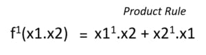
• Product Rule

The product rule states that if we have a function in the form of f(x).g(x), then we can find the derivative very easily by applying the rule as shown below. I will not show you an example because it becomes too complicated. You can find various resources online to know more.

• Chain Rule

The chain rule states that if we have embedded functions such as of the form: f(g(x)), then we can easily find the derivative of this function by the following rule:

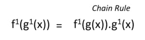
These are all the rules that you need to remember for using calculus in Machine Learning. The next step? Practice as much as you can to get the hang of using these rules. As promised, I have written down some of the most repeated functions that you can go through as a cheat-sheet in solving such problems.

Now that we have finally learnt all there is to learn about differentiation, let’s extend this concept. It’s time to move to something that is realistic and used in real-life by many in the industry.

3.3 Partial Differentiation

Partial Differentiation is an important concept that most of us have ignored all through our academy. ‘What has Partial Differentiation helped us achieve?’ is the question most of you would be having right now. Let me give you an example so that you can understand the importance.

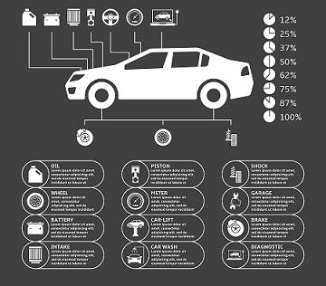
Suppose you are a car designer. There are so many factors that you would want to change in the body of your car so that you are able to provide the best possible performance. What are you going to vary? The engine and other internal parts? No! You are going to change the body of the car. You vary the design, add or delete various windshields, air intake and outtakes and all there is that comes to when you are a designer.

When you are the tuner of the car, you don’t change the body and other parameters. You just change the internal parts such as the engine and all that is there so that you can make the car give the most optimal performance.

So what did you understand from this example?

Summing it up, you vary only certain parameters that you are interested in and not the other parts of the car. Only differentiate what you want to and other parameters remain constant. That is what Partial Differentiation is.

Of course, this is a very bland example but in reality, this is the same logic that is followed. You vary some parameters and differ others so that you can obtain the most optimal performance. If an engine is to be tuned, you vary the oil intake while keeping other parts constant and see the performance. Simple enough to understand right?

But, what is the difference between Differentiation and Partial Differentiation? The answer is just the way you work with the parameters. One point to note here is that Differentiation has just one variable that you differ, whereas there are many variables when it comes to Partial Differentiation.

Still, confused? Let me show you the equation that makes Partial Differentiation.

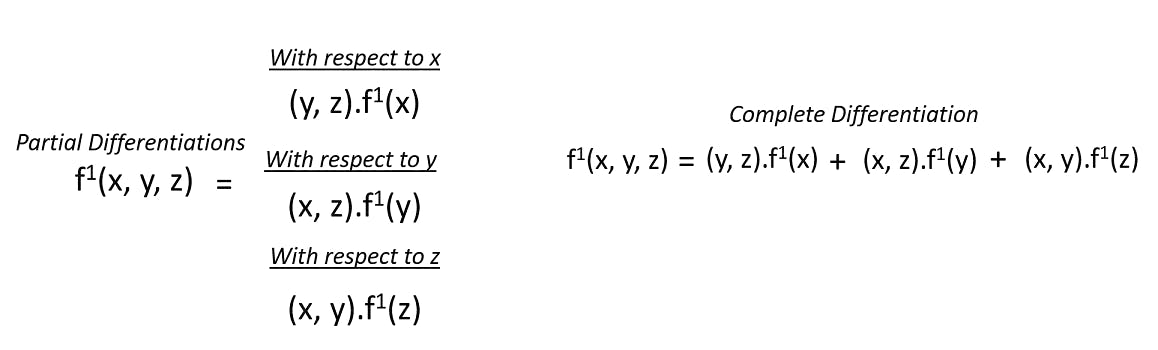
Let’s solve a small example so that you can understand how Partial Differentiation really works. Let’s assume that our equation here is:

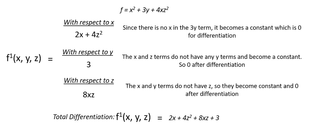
With this, you can understand what exactly has happened. The y term does not contribute to anything and the equation is truly dependent on x and z terms only. They help us to derive something that we are searching for through the equation.

Now that we have a clear understanding of what is Partial Differentiation and why it is such an important part of the real world computations, let’s jump right into the real scenario that we face in Machine Learning, the applications of Multivariate Calculus in Machine Learning!

3.4 Application of Multivariate Calculus in Machine Learning

Multivariate Calculus has found a firm grip of itself in the field of Machine Learning. It is capable of helping us optimize our models, used in Deep Learning, finding errors and so much more. Let’s discuss it all now.

• The Jacobian is a vector matrix of the first order derivatives which points to the maximum global value in the dataset. The Jacobian is also capable of linearizing a nonlinear function by which we are able to apply a standard function that can be applied to a linear type

• The Hessian is a vector matrix of the second-order derivatives. It plays a huge factor in linear algebra and helps to iteratively help find the minimum error that can be obtained in the function outputs.

• Gradient Descent helps us find optimal weights of the equation such that we are able to find the best output for our problems. We start with Random weights, find the minimum error between points and optimize the model.

• They are also used in making Deep Learning Models.

Now that we know the applications, we need to know how this happens in real life. Here is a practical application where Multivariate Calculus is used in the optimization of the output for the model that we create.

So this brings us to the end of all that is required from Multivariate Calculus in the field of Mathematics for Machine Learning. I hope Linear Algebra and Multivariate Calculus have been easy to understand and visualize efficiently.

4. Probability

Probability, the heart of assumptions. What do I mean by that? Well, when you assume something, there is always a probability or chance of that assumption happening. But how do we put that into Mathematical Terms? That’s where probability comes to help us.

Probability is also the reason we make assumptions, hypothesis and more. So it plays a really important role when it comes to Mathematics for Machine Learning. So sit tight as we are now going to understand all the required math in probability.

4.1 What is Probability?

Probability in the simplest of explanations is the chance of something happening but in a quantified manner. Meaning that there is a number that is attached to something happening. When I say let’s flip a coin, there is an equal chance of it being either a head or a tail. So if we put this into numbers, there is a 50% chance that it could be either a head or a tail.

In the formal sense, “Probability is a measure of how likely an event will occur.” It can be written down as:

Probability = Event Desired / Total Outcomes

Suppose we have a deck of cards, out of which we need to find out the probability that the card we pull out is a heart. We know that there are 52 cards in a deck. 13 cards of hearts, club, spades and diamonds each. That means there are 13 cards which we favour and 52 cards are the total cards. So the probability is calculated as:

13/52 = 1/4 = 0.25

That is how we find out the probability. Now that we have understood what is Probability and how to find it, let’s dive deeper into the roots and understand all the needed information that we need.

4.2 Terminologies in Probability

Before diving deep into the concepts of probability, it is important that you understand the basic terminologies used in probability:

• Random Experiment: An experiment or a process for which the outcome cannot be predicted with certainty.

• Sample space: The entire possible set of outcomes of a random experiment is the sample space of that experiment.

• Event: One or more outcomes of an experiment is called an event. It is a subset of sample space. There are two types of events in probability:

Disjoint Event: Disjoint Events do not have any common outcomes. For example, a single card drawn from a deck cannot be a king and a queen

Joint Event: Non-Disjoint Events can have common outcomes. For example, a student can get 100 marks in statistics and 100 marks in probability

4.3 Distributions in Probability

Probability Distributions help us understand the kind of data we are working with, how they are distributed and differ from each other. Every aspect of the data can be understood, visualized using the Distributions.

For Machine Learning, we will only concentrate on 3 distributions:

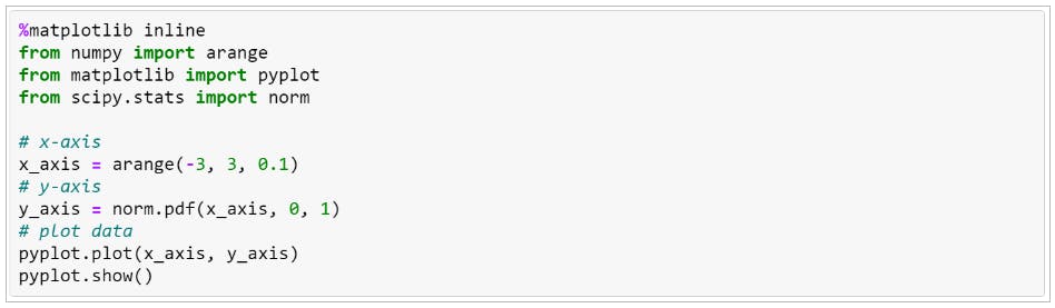
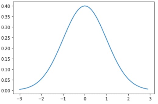
1. Probability Density Function (PDF) is concerned with the relative likelihood for a continuous random variable to take on a given value. The PDF gives the probability of a variable that lies between the range ‘a’ and ‘b’.

2. Normal Distribution is a probability distribution that denotes the symmetric property of the mean. It infers that the data around the mean represents the entire data set.

3. Central Limit Theorem states that the sampling distribution of the mean of any independent, random variable will be normal or nearly normal if the sample size is large enough. To read more about them, I have this article here that will help you out better. Once we are clear with the Distributions, let’s talk about the types of Probability.

4.4 Types of Probability

Probability depends on the kind of application we are working with. There are basically 3 types of Probability that we have:

1. Marginal Probability means that an event will occur without any intervention or dependency on others.

2. Joint Probability is a measure of two events happening at the same time.

3. Conditional Probability is the measure that an event will occur only if some other event has already occurred. It is dependent on the previous event.

For in-depth knowledge on types of Probability, you can follow this link. So now that we have that out of the way, let’s move over to the most important topic in Probability, Bayes’ Theorem.

4.5 Bayes’ Theorem

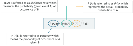
The Bayes theorem is used to calculate the conditional probability. It is the probability of an event occurring based on prior knowledge of conditions that might be related to the event. The formula for Bayes Theorem goes something like this:

4.6 Application of Probability in Machine Learning

By now, all of us have a clear idea of the impact Probability has on Machine Learning but the real question as always remains. How do we use this in real life? Well, let’s talk about that now.

• Probability helps us optimize our model
• Classification by our algorithms requires Probability
• Loss can also be calculated using Probability
• Models are built on Probability

Here is a practical application of Naive Bayes Classifier that requires Probability and how it helps us in making a good model. The graphic image below is another example of how the Naive Bayes Classifier works.

With that, we have now covered everything there is for Probability in the field of Machine Learning. Let’s move over to Statistics in Machine Learning.

5. Statistics

Statistics is an important factor when it comes to Machine Learning. It is a tool that helps you study, analyze and make work out of the Hypothesis you make that will be able to predict. So without waiting anymore, let’s learn all there is!

5.1 What is Statistics?

Statistics is an area of applied mathematics concerned with data collection, analysis, interpretation, and presentation. It helps you in testing the effectiveness of your Hypothesis on the dataset that you have gathered. That makes it such an important factor in Machine Learning.

5.2 Basic Terminologies in Statistics

Statistics revolves around data. So understanding what the terms mean comes to be a very important factor in this. There are basically 2 things that you need to remember.

1.Population: A collection or set of individuals or objects or events whose properties are to be analyzed

2.Sample: A subset of the population is called ‘Sample’. A well-chosen sample will contain most of the information about a particular population parameter

As you can see from the figure above, we have a whole population of fish which is the whole dataset. From that, we choose a set that represents the population best. I hope this example helps you understand these rather simple terms.

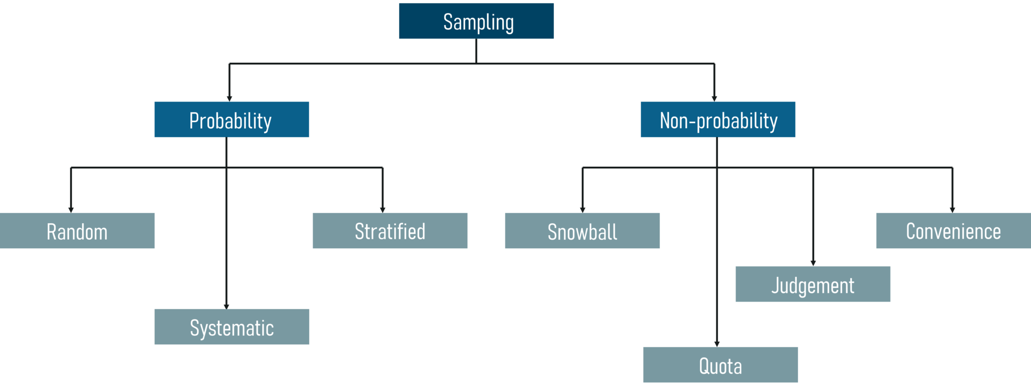
5.3 Sampling Techniques

Sampling is the process of selecting your samples from the whole population of data. But the sample should be efficient enough so that it is able to help you tell everything there is about the data. But how do we do that? There are a few approaches:

5.4 Types of Statistics

There are basically 2 kinds of Statistics when it comes to Mathematics. We have:

1. Descriptive Statistics – This is when you are trying to describe the kind of data you are working with. It describes what the data has, what it covers, and much more.

2. Inferential Statistics – This is when you are trying to infer some knowledge or information from the data. Suppose you make a hypothesis and test that, you get back some inference from that. Let’s now move over to Hypothesis Testing.

5.5 Hypothesis Testing

The first thing that pops up in our minds is, “What is a Hypothesis?”. Well, remember the assumptions that I was talking about before while talking about Probability, those assumptions are what we call a Hypothesis. We make a situation or a statement that could be a possibility of happening.

You may wonder how do these assumptions come in line with Statistics? Well, we use Statistics to test whether these Hypotheses are right or not. This article here will help you understand all there is to know about Hypothesis Testing.

And with that, we have come to the end of Statistics in Machine Learning. I hope everything has become clear to you guys and with that, let’s wrap up this long ride.

5.6 Population and Sample

• Population:

In statistics, the population comprises all observations (data points) about the subject under study.

An example of a population is studying the voters in an election. In the 2019 Lok Sabha elections, nearly 900 million voters were eligible to vote in 543 constituencies.

• Sample:

In statistics, a sample is a subset of the population. It is a small portion of the total observed population.

An example of a sample is analyzing the first-time voters for an opinion poll.

• Measures of Central Tendency

Measures of central tendency are the measures that are used to describe the distribution of data using a single value. Mean, Median and Mode are the three measures of central tendency.

• Mean:

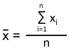
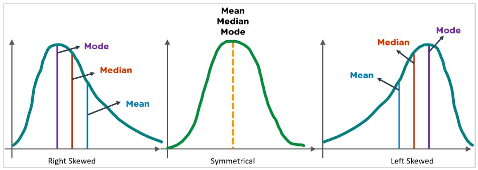
The arithmetic mean is the average of all the data points.

If there are n number of observations and xi is the ith observation, then mean is:

Consider the data frame below that has the names of seven employees and their salaries.

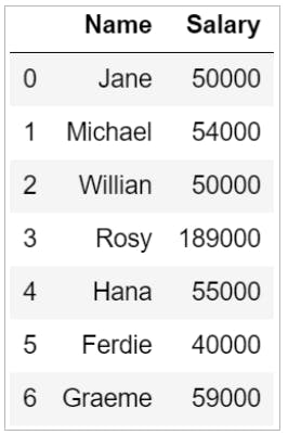
To find the mean or the average salary of the employees, you can use the mean() functions in Python.

• Median:

Median is the middle value that divides the data into two equal parts once it sorts the data in ascending order.

If the total number of data points (n) is odd, the median is the value at position (n+1)/2.

When the total number of observations (n) is even, the median is the average value of observations at n/2 and (n+2)/2 positions.

The median() function in Python can help you find the median value of a column. From the above data frame, you can find the median salary as:

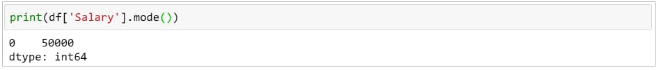
• Mode: The mode is the observation (value) that occurs most frequently in the data set. There can be over one mode in a dataset.

Given below are the heights of students (in cm) in a class:

155, 157, 160, 159, 162, 160, 161, 165, 160, 158

Mode = 160 cm.

The mode salary from the data frame can be calculated as:

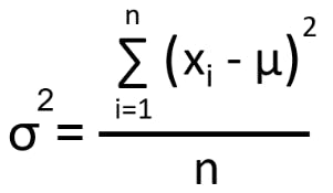
• Variance and Standard Deviation

Variance is used to measure the variability in the data from the mean.

Consider the below dataset.

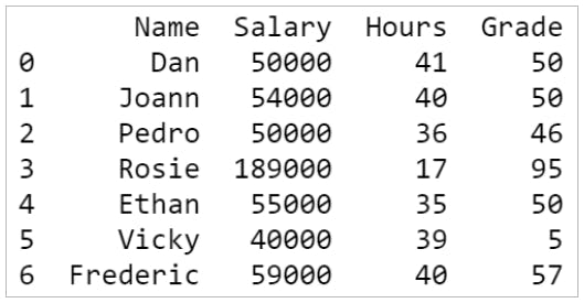
To calculate the variance of the Grade, use the following:

Standard deviation in statistics is the square root of the variance. Variance and standard deviation represent the measures of fit, meaning how well the mean represents the data.

You can find the standard deviation using the std() function in Python.

• Range and Interquartile Range

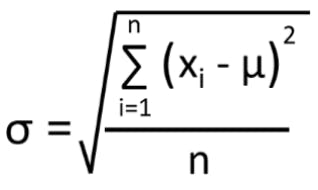
• Range:

The Range in statistics is the difference between the maximum and the minimum value of the dataset.

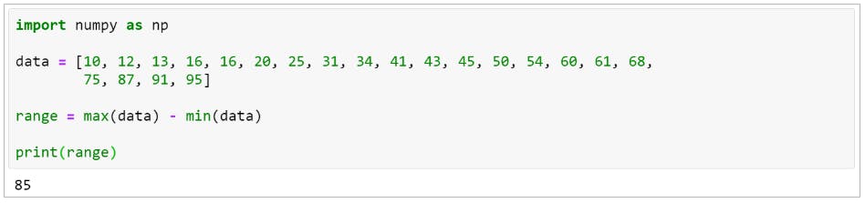
• Interquartile Range (IQR) :

The IQR is a measure of the distance between the 1st quartile (Q1) and 3rd quartile (Q3).

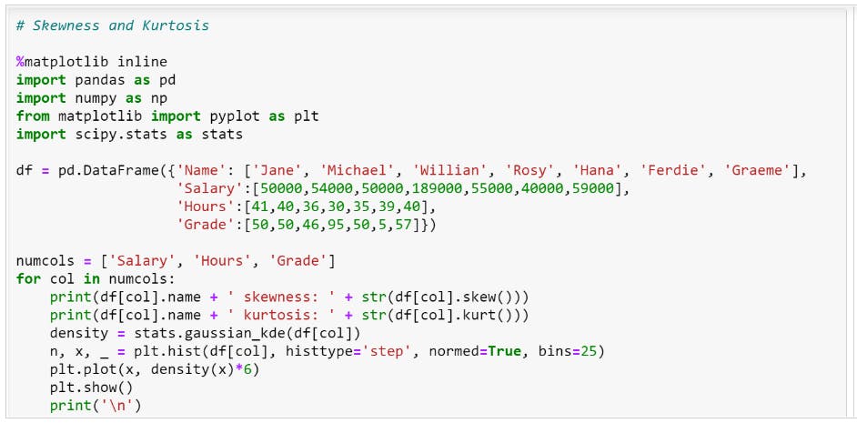
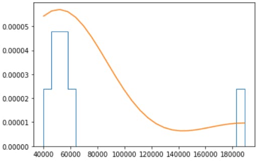
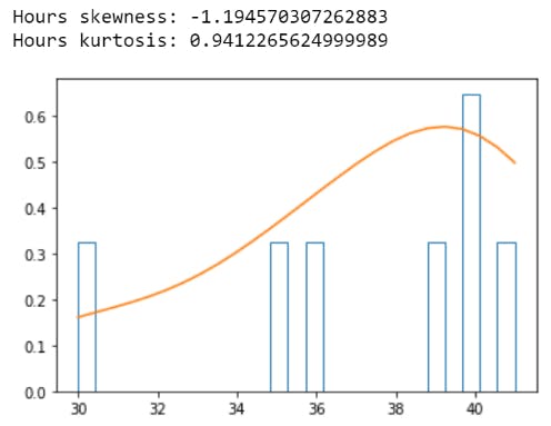
• Skewness and Kurtosis

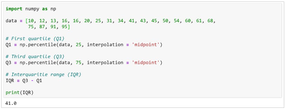
• Skewness:

Skewness measures the shape of the distribution. A distribution is symmetrical when the proportion of data at an equal distance from the mean (or median) is equal. If the values extend to the right, it is right-skewed, and if the values extend left, it is left-skewed.

Kurtosis:

Kurtosis in statistics is used to check whether the tails of a given distribution have extreme values. It also represents the shape of a probability distribution.

Gaussian Distribution

In statistics and probability, Gaussian (normal) distribution is a popular continuous probability distribution for any random variable. It is characterized by 2 parameters (mean μ and standard deviation σ). Many natural phenomena follow a normal distribution, such as the heights of people and IQ scores.

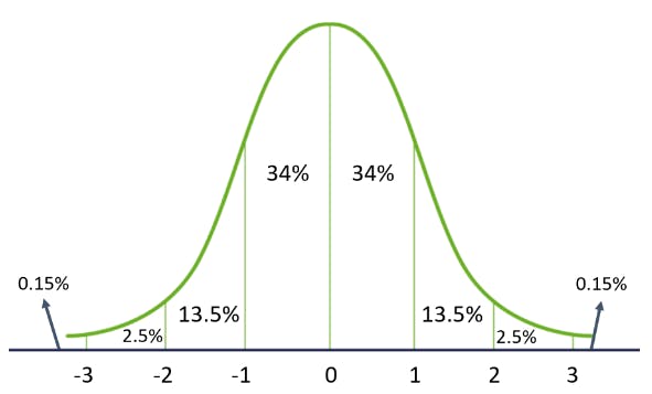
• Properties of Gaussian Distribution:

• The mean, median, and mode are the same

• It has a symmetrical bell shape
• 68% data lies within 1 standard deviation of the mean
• 95% data lie within 2 standard deviations of the mean
• 99.7% of the data lie within 3 standard deviations of the mean

• Central Limit Theorem

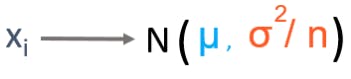
According to the central limit theorem, given a population with mean as μ and standard deviation as σ, if you take large random samples from the population, then the distribution of the sample means will be roughly normally distributed, irrespective of the original population distribution.

Rule of Thumb: For the central limit theorem to hold true, the sample size should be greater than or equal to 30.

6. Pavlov trained experiment his dog using reinforcement training

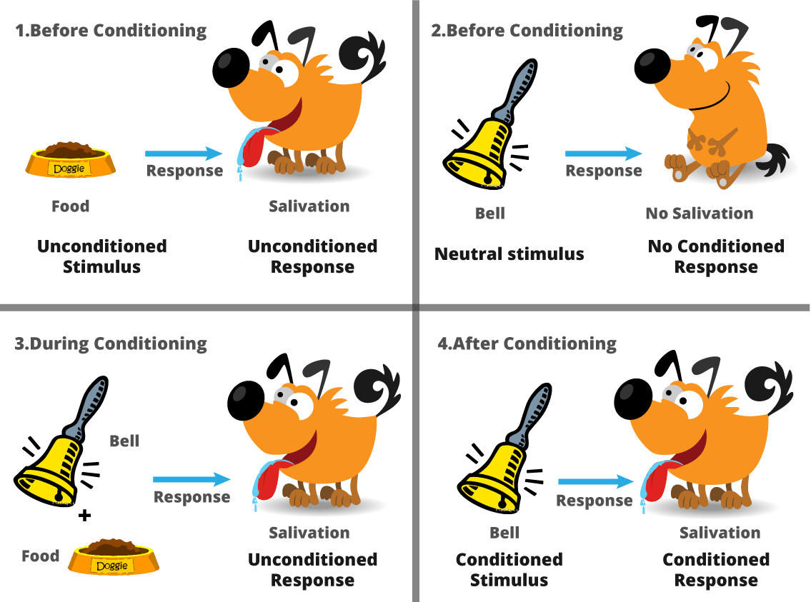
Pavlov divided the training of his dog into four stages.

In the first part, Pavlov gave meat to the dog, and in response to the meat, the dog started salivating.

In the next stage he created a sound with a bell, but this time the dogs did not respond anything.

In the third stage, he tried to train his dog by using the bell and then giving them food. Seeing the food the dog started salivating.